Performance¶

Goals¶

pysorteddict was performance-benchmarked in order to:

evaluate it under synthetic workloads targeting the specific features it provides; and
understand how well the underlying data structure (typically a red-black tree) handles those workloads.

Nonetheless, the results should still be broadly indicative of real-world performance.

Environment¶

Component	Specification
CPU	Intel Core i9-12900H
CPU Frequency Scaling Governor	powersave
RAM	16 GiB DDR5
Kernel	Linux 6.12.74 (64-bit)
Operating System	Debian 13 “trixie”
Operating System Libraries	GNU C Library 2.41, GNU C++ Library 14.2.0
Python Interpreter	CPython 3.13.5
Python Interpreter Libraries	pysorteddict 0.14.0

Strategy¶

The key type chosen was float, since it is easy to generate floating-point numbers uniformly distributed in the unit interval. Comparing two floats is straightforward (as opposed to comparing, say, two strs—if their lengths are different, they may introduce noise in the benchmarks). Before every benchmark, the random number generator was seeded with π, a nothing-up-my-sleeve number.

The performance benchmarking code is in a Jupyter notebook in the GitHub repository. It contains everything required to generate the data and graphs on this page.

Results¶

Lookup¶

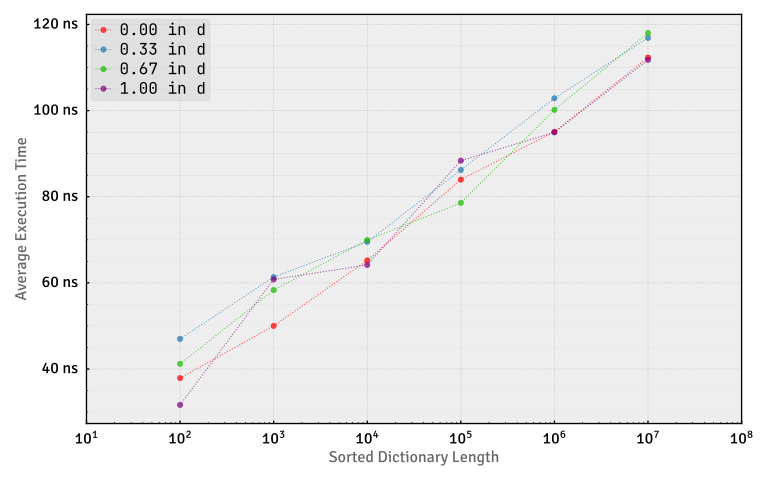
The numbers 0.00, 0.33, 0.67 and 1.00 are spaced equally in the range spanned by the keys, but are absent in the sorted dictionaries constructed using the seeded random number generator described above. Hence, a search for them in the red-black tree backing any pysorteddict.SortedDict will not terminate permaturely.

Insertion and Deletion¶

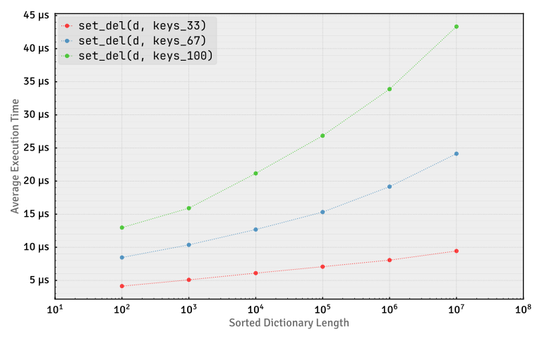
Inserting or deleting an item into or from a sorted dictionary changes its length. Hence, benchmarks which only insert or only delete items cannot be said to have been performed on a sorted dictionary of a particular length. Therefore, the strategy chosen was:

generate a list of random floats;
insert all of them into the sorted dictionary; and
delete all of them from the sorted dictionary in order of insertion.

Only the last two steps (defined in a function set_del) were timed. After these, ideally, the sorted dictionary should return to the original state, allowing it to be used for the next round of timing. In practice, it is likely to be in a different state because of rebalancing operations. But that change of state can be assumed to simulate the real-world effects of insertions and deletions, so this is a sound strategy.

This benchmark was repeated for four different lengths of the list of random floats: 100, 200, 300 and 400.

Batch Insertion and Deletion¶

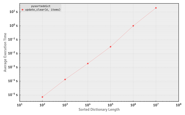
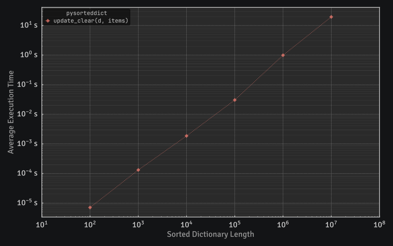
Extending the logic of the previous benchmark, the strategy here was:

generate a list of tuples of random floats and None;
update the sorted dictionary with them; and
clear the sorted dictionary.

In effect, this benchmark indicates the time taken to populate and empty a sorted dictionary.

Iteration¶

Data¶

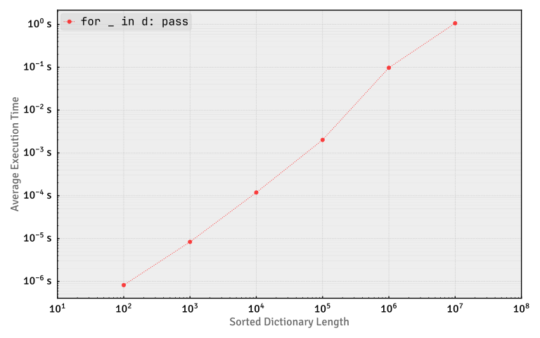
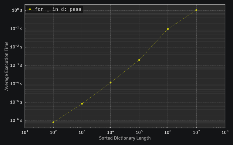
The benchmark data used to plot the above graphs is tabulated below.

Expression	Sorted Dictionary Length
Expression	10²	10³	10⁴	10⁵	10⁶	10⁷
`0.00 in d`	40.2 ns	52.9 ns	69.1 ns	90.0 ns	109 ns	121 ns
`0.33 in d`	47.9 ns	66.5 ns	72.6 ns	89.6 ns	107 ns	122 ns
`0.67 in d`	41.6 ns	60.5 ns	73.0 ns	82.1 ns	107 ns	123 ns
`1.00 in d`	30.6 ns	60.4 ns	64.3 ns	84.7 ns	101 ns	117 ns
`set_del(d, keys_100)`	13.3 μs	18.1 μs	24.6 μs	31.7 μs	39.3 μs	49.6 μs
`set_del(d, keys_200)`	32.6 μs	42.9 μs	58.5 μs	73.9 μs	94.1 μs	164 μs
`set_del(d, keys_300)`	55.9 μs	69.5 μs	91.0 μs	116 μs	189 μs	344 μs
`set_del(d, keys_400)`	79.9 μs	96.5 μs	124 μs	165 μs	293 μs	483 μs
`update_clear(d, items)`	7.09 μs	132 μs	1.86 ms	30.4 ms	986 ms	19.5 s
`for _ in d: pass`	607 ns	6.09 μs	98.2 μs	1.75 ms	99.6 ms	1.29 s
`for _ in reversed(d): pass`	834 ns	8.10 μs	124 μs	2.72 ms	107 ms	1.32 s